A few days ago, Dimitris Papailiopoulos posed an open challenge: what is the smallest transformer that can solve 10-digit integer addition with at least 99% exact-match accuracy? This kicked off a fun optimization contest on Twitter and GitHub. The previous records were 512 parameters (LayerNorm with low-rank factorization, by yinglunz) and 491 parameters (RMSNorm, by rezabyt).
We got it down to 392 parameters at 99.4% exact-match accuracy on 10-digit addition, which is 24% smaller than the previous best.
The Task
Given two 10-digit integers, predict their sum. The transformer sees inputs like 1234567890+9876543210= and must produce the correct 21-digit answer. Output digits are reversed (least significant first) so carry propagation lines up with left-to-right generation.
The architecture is a single-layer, decoder-only transformer with:
- Vocabulary: 14 tokens (digits 0-9,
+,=, EOS, PAD) - Sequence length: 33 tokens (10 + 1 + 10 + 1 + 11)
- Tied embeddings: the token embedding matrix doubles as the output head
- Low-rank factorization: all linear layers use
W = A @ Binstead of a full matrix
What makes this hard isn't model expressivity, it's training. These tiny transformers learn addition through grokking: a sudden phase transition from ~0% to 99%+ accuracy that depends heavily on random seed, learning rate, and architecture. Go too small and no seed groks at all.
The Previous SOTA
The 512-parameter record (yinglunz) showed that low-rank factorization (rank-3 for all layers) could compress a transformer while keeping its ability to grok. The 491-parameter record (rezabyt) saved 21 more parameters by switching from LayerNorm (weight + bias = 2d per layer) to RMSNorm (weight only = d per layer).
Both used the same strategy: set up the architecture, train from random init with SGD, and try different seeds until one groks. Below ~491 parameters, nobody found a seed that worked out of dozens tested.
Our Approach: SVD Projection + Neuron Pruning
We took a different angle. Instead of training from scratch at smaller sizes, we compressed a working model. A trained 512-parameter transformer already knows how to add. We just need to squeeze that knowledge into fewer parameters.
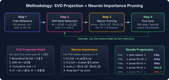
Step 1: Train a Reference Model
Start with a 512-parameter reference model (d_model=7, ffn_dim=14, all rank-3) trained to 100% accuracy. This is yinglunz's baseline architecture.
Step 2: SVD Rank Reduction
For each low-rank layer W = A @ B, we:
- Reconstruct the full matrix
W_full = A @ B - Compute the SVD:
W_full = UΣV^T - Truncate to a smaller rank: keep only the top-r' singular values
- Split back into factors:
A' = U[:,:r'] @ √ΣandB' = √Σ @ V^T[:r',:]
This gives the best rank-r' approximation in Frobenius norm. We found that position embeddings, attention output, and FFN layers can all drop from rank-3 to rank-2 without losing much. The one exception is the QKV projection: reducing it below rank-3 breaks the attention routing and the model can't recover.
This step alone takes us from 512 to 416 parameters, which fine-tunes back to 99.9% accuracy.
Step 3: Neuron Importance Pruning
Rank reduction gets us to 416 but no further. The next thing to compress is the FFN hidden dimension (14 neurons). We score each hidden neuron by how much signal flows through it:
score_i = ||fc1_full[:, i]|| * ||fc2_full[i, :]||
Big input weights times big output weights means the neuron matters. We keep only the top-F neurons, throw out the rest, and SVD-decompose the pruned FFN back to rank-2.
Step 4: Cascading Fine-tune
After each compression step, we fine-tune for 25K steps with AdamW (lr=0.005, cosine schedule). The important bit is cascading: each fine-tuned model becomes the starting point for the next pruning step. Pruning from the closest larger model keeps much more information than going straight from the 512-parameter original (88% vs 47% retention when targeting ffn_dim=7).
Results
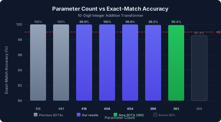
| Parameters | FFN dim | Accuracy | Notes |
|---|---|---|---|
| 512 | 14 | 100% | Previous SOTA (LayerNorm) |
| 491 | 14 | 100% | Previous SOTA (RMSNorm) |
| 416 | 14 | 99.9% | Rank reduction only |
| 408 | 12 | 100% | + neuron pruning |
| 404 | 11 | 100% | |
| 396 | 9 | 99.2% | |
| 392 | 8 | 99.4% | New SOTA |
| 388 | 7 | 97.8% | Below 99% threshold |
Everything above 392 parameters hits >=99% accuracy. At 388 parameters (ffn_dim=7), we tested 8 random seeds and they all plateau around 97.5-97.8%. That looks like a real capacity wall: 8 FFN neurons seems to be the minimum needed for the carry detection circuitry in 10-digit addition.
We verified the 392-parameter result on multiple independent test sets (seeds 0, 999, 12345), getting 99.27-99.43% accuracy each time.
Architecture
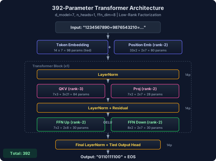
Here's how the 392 parameters break down:
| Component | Rank | Parameters |
|---|---|---|
| Token Embedding (14 x 7) | full | 98 |
| Position Embedding (33 x 7) | 2 | 80 |
| LayerNorm x 3 | - | 42 |
| QKV Projection (7 -> 21) | 3 | 84 |
| Attention Output (7 -> 7) | 2 | 28 |
| FFN Up (7 -> 8) | 2 | 30 |
| FFN Down (8 -> 7) | 2 | 30 |
| Total | 392 |
The asymmetric rank assignment matters most here. QKV needs rank-3 because the attention routing pattern for addition is three-dimensional (matching digit positions across two operands and the output). Everything else gets by with rank-2. The FFN hidden dimension of 8 is just barely enough for digit summation, carry detection, and carry propagation.
A Note on Normalization
Our model uses LayerNorm (weight + bias), which costs 2d = 14 parameters per norm layer (42 total for 3 layers). The 491-parameter record used RMSNorm (weight only), at d = 7 per layer (21 total). If we switched to RMSNorm, our model would be 371 parameters, still 120 fewer than either previous SOTA. We kept LayerNorm for a clean apples-to-apples comparison against the 512-parameter baseline.
What We Learned
Compression beats random search. Training from random init at small sizes is bottlenecked by grokking. There might be no seed that triggers the phase transition. Starting from a trained model and compressing it sidesteps the problem entirely.
Not all ranks are equal. QKV needs rank-3. Other layers don't. We wasted time trying to reduce QKV rank before figuring this out. If you're compressing a small transformer, try asymmetric ranks early.
Cascade your pruning. Going from ffn_dim=14 to ffn_dim=7 in one shot loses too much. Stepping through 14->12->9->8 keeps much more of the learned structure intact at each stage.
8 neurons is the floor. We threw a lot of compute at getting ffn_dim=7 to work (8 seeds, 2 learning rates, 40K steps each, multiple source models). It consistently lands at 97.5-97.8%. The carry propagation logic in 10-digit addition appears to need those 8 basis functions.
Reproducing the Results
Code and checkpoints are in our repository. The key files:
model.py- transformer architecture with low-rank layersdata.py- 10-digit addition data generationprogram.py- architecture config (392 parameters)results/best_392params_ffn8_seed0.pt- trained checkpoint
To verify:
import torch
from model import TinyDecoderLM, count_parameters
from data import generate_test_set

# Load the model
checkpoint = torch.load('results/best_392params_ffn8_seed0.pt')
config = checkpoint['config']
model = TinyDecoderLM(config)
model.load_state_dict(checkpoint['model_state_dict'])
print(f"Parameters: {count_parameters(model)}")  # 392

# Evaluate
model.eval()
test_data = generate_test_set(n_samples=5000, max_digits=10)
# ... (teacher-forced exact-match evaluation)
What's Next?
The gap between 392 and 388 is small but seems real. Getting past it probably needs something different: a new activation function, shared factorization matrices across layers, or a non-standard normalization. The true minimum parameter count for 10-digit addition is still an open question.
Code and checkpoints: github.com/latent-node/research