Distributed Training on Heterogeneous Macs

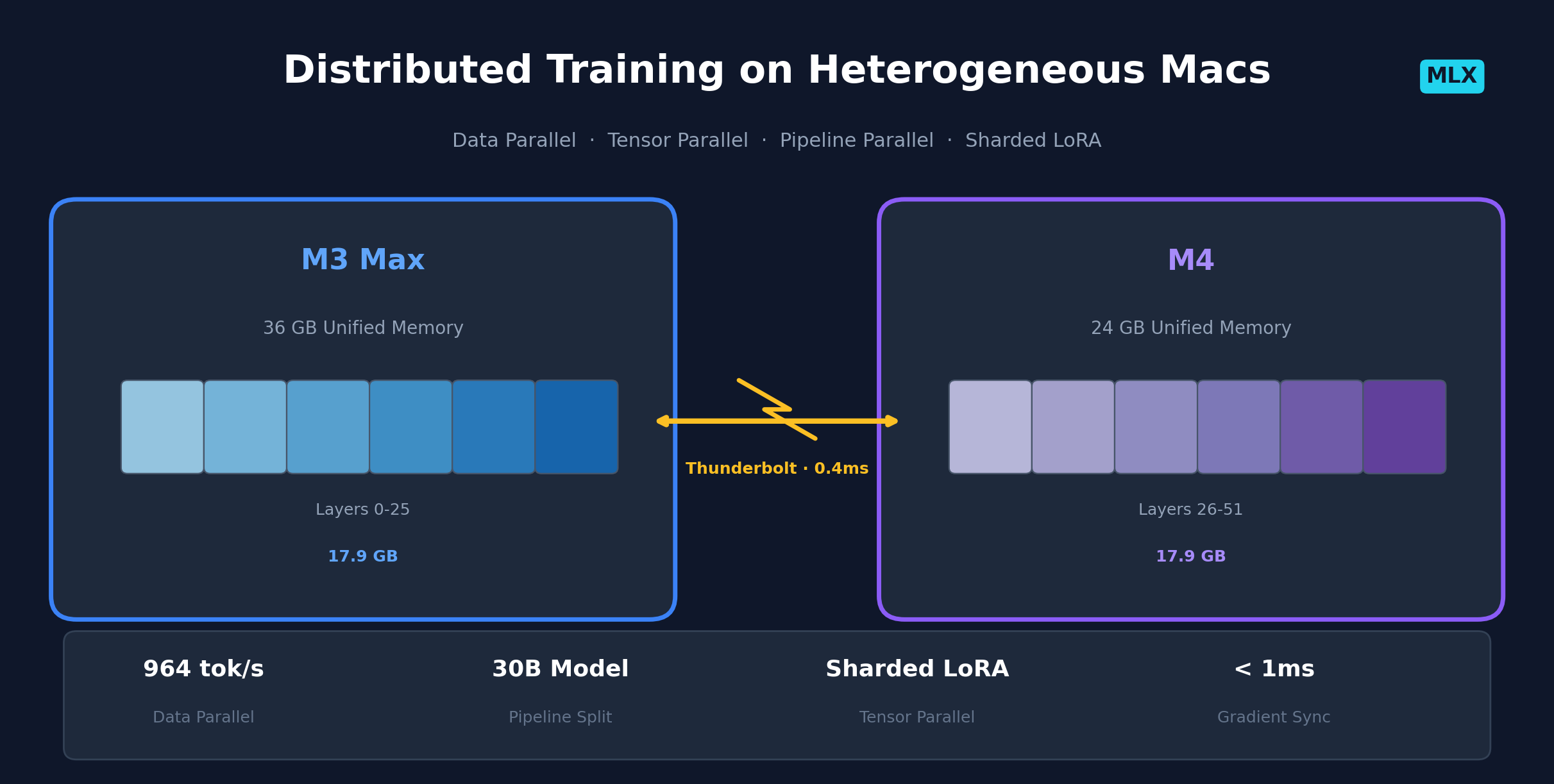
How we connected an M3 Max and an M4 MacBook Pro over Thunderbolt, built a distributed training cluster, and implemented sharded LoRA for tensor-parallel fine-tuning.

Most guides to distributed ML training assume you have identical hardware. Matching Mac Minis in a rack. A fleet of Mac Studios with the same chip and memory. We had two MacBook Pros sitting on a desk, connected by a Thunderbolt cable. One has an M3 Max with 36 GB of unified memory. The other has an M4 with 24 GB. Different chips, different memory, different usernames, different home directories.

This guide covers making that work in practice, sharp edges and all. By the end, we had data-parallel QLoRA fine-tuning running 2x faster across both machines, tensor-parallel inference splitting models across nodes, and a sharded LoRA implementation that lets you fine-tune models too large for either Mac alone.

The Hardware

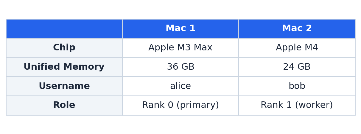
A Thunderbolt cable connects the two machines directly. Round-trip latency: 0.4 ms. The same machines over WiFi: 20-300 ms with jitter. For gradient synchronization during training, that gap changes everything.

Setting Up the Network: The Bridge0 Story

macOS manages Thunderbolt Ethernet interfaces through a software bridge called bridge0. When you plug in a Thunderbolt cable between two Macs, macOS automatically bridges the underlying interfaces (en1, en2, en3) and assigns link-local IPv4 addresses (169.254.x.x) to bridge0 on each machine.

First important lesson: always work with bridge0, never with the underlying interfaces directly.

To find your bridge0 IPs after connecting the cable:

# On each Mac
ifconfig bridge0 | grep "inet "

You'll see something like inet 169.254.142.41 on one machine and inet 169.254.116.127 on the other. These addresses change after every reboot, so you'll need to check them each time.

We learned this the hard way. Early on, we followed mlx.distributed_config's suggestion to take down bridge0 and assign static IPs directly to en1/en2. Ping succeeded between the machines. TCP connections silently failed with EHOSTUNREACH errors. ICMP packets flowed fine. TCP did not.

The root cause: removing an interface from bridge0 with ifconfig bridge0 deletem en1 puts macOS's network stack into an inconsistent state where the kernel's TCP path disagrees with its ICMP path about how to route packets through the Thunderbolt interface. The only fix is a full reboot.

Never run ifconfig bridge0 deletem on a Thunderbolt interface. It breaks TCP and requires a reboot to fix. We spent hours on this. Ping works. Every TCP connection returns error 65 (EHOSTUNREACH).

Setting Up SSH

mlx.launch uses SSH to start processes on remote machines. You need passwordless SSH between both Macs. Both directions, if you want mlx.distributed_config to work.

# Add your key to the agent (persists across reboots on macOS)
ssh-add --apple-use-keychain ~/.ssh/id_rsa

# Copy your public key to the other Mac
ssh-copy-id bob@mac2.local

# Also set up SSH to localhost (needed by mlx.distributed_config)
ssh-copy-id 127.0.0.1

If your SSH key has a passphrase and you skip the --apple-use-keychain flag, the key gets forgotten after every reboot. The flag stores the passphrase in macOS Keychain so it persists. Add this to ~/.ssh/config to make it automatic:

Host *
    AddKeysToAgent yes
    UseKeychain yes

One more thing: the other Mac may need someone to log in at the physical login screen before SSH becomes available. FileVault blocks SSH until the first user login after boot.

The Hostfile

MLX's ring backend needs a JSON hostfile that maps SSH hostnames to IP addresses. For our two-Mac setup:

[
    {"ssh": "127.0.0.1", "ips": ["169.254.142.41"]},
    {"ssh": "bob@mac2.local", "ips": ["169.254.116.127"]}
]

The first entry uses 127.0.0.1 for the local machine. The ring backend checks for this exact string to identify the local process and run it directly instead of SSH-ing to itself.

The IPs must be the bridge0 addresses (the Thunderbolt link), not WiFi. Using WiFi IPs would work but at 50-100x higher latency.

Since bridge0 IPs change after every reboot, we keep a script to regenerate the hostfile:

LOCAL_IP=$(ifconfig bridge0 | grep "inet " | awk '{print $2}')
REMOTE_IP=$(ssh bob@mac2.local "ifconfig bridge0 | grep 'inet '" | awk '{print $2}')
cat > hosts_tb.json << EOF
[
    {"ssh": "127.0.0.1", "ips": ["$LOCAL_IP"]},
    {"ssh": "bob@mac2.local", "ips": ["$REMOTE_IP"]}
]
EOF

The Different-Paths Problem

Our two Macs have different usernames, which means different home directories:

• Mac 1: /Users/alice/projects/dist-mlx/
• Mac 2: /Users/bob/projects/dist-mlx/

This creates a practical problem: mlx.launch resolves script paths to absolute paths on the launching machine, then tries to run the same absolute path on the remote machine. /Users/alice/... doesn't exist on Mac 2.

The solution is a combination of two flags:

.venv/bin/mlx.launch --backend ring --hostfile hosts_tb.json \
  --python .venv/bin/python3 \
  --cwd projects/dist-mlx \
  -p 3700 \
  /tmp/my_script.py

• --cwd projects/dist-mlx changes the working directory on each node. Since this is a relative path from the home directory, it resolves correctly on both machines.
• --python .venv/bin/python3 uses a relative Python path that works with --cwd.
• Scripts go in /tmp/ which exists at the same path on both machines.
• -p 3700 sets a custom starting port (useful if the default port 2700 has a stale binding after a previous run).

Before launching, copy the script to both machines:

cp my_script.py /tmp/my_script.py
scp my_script.py bob@mac2.local:/tmp/my_script.py

Data-Parallel Training

Data parallelism is the simplest form of distributed training. Each machine holds a complete copy of the model. Each processes a different shard of the data. Gradients are averaged across machines after each step.

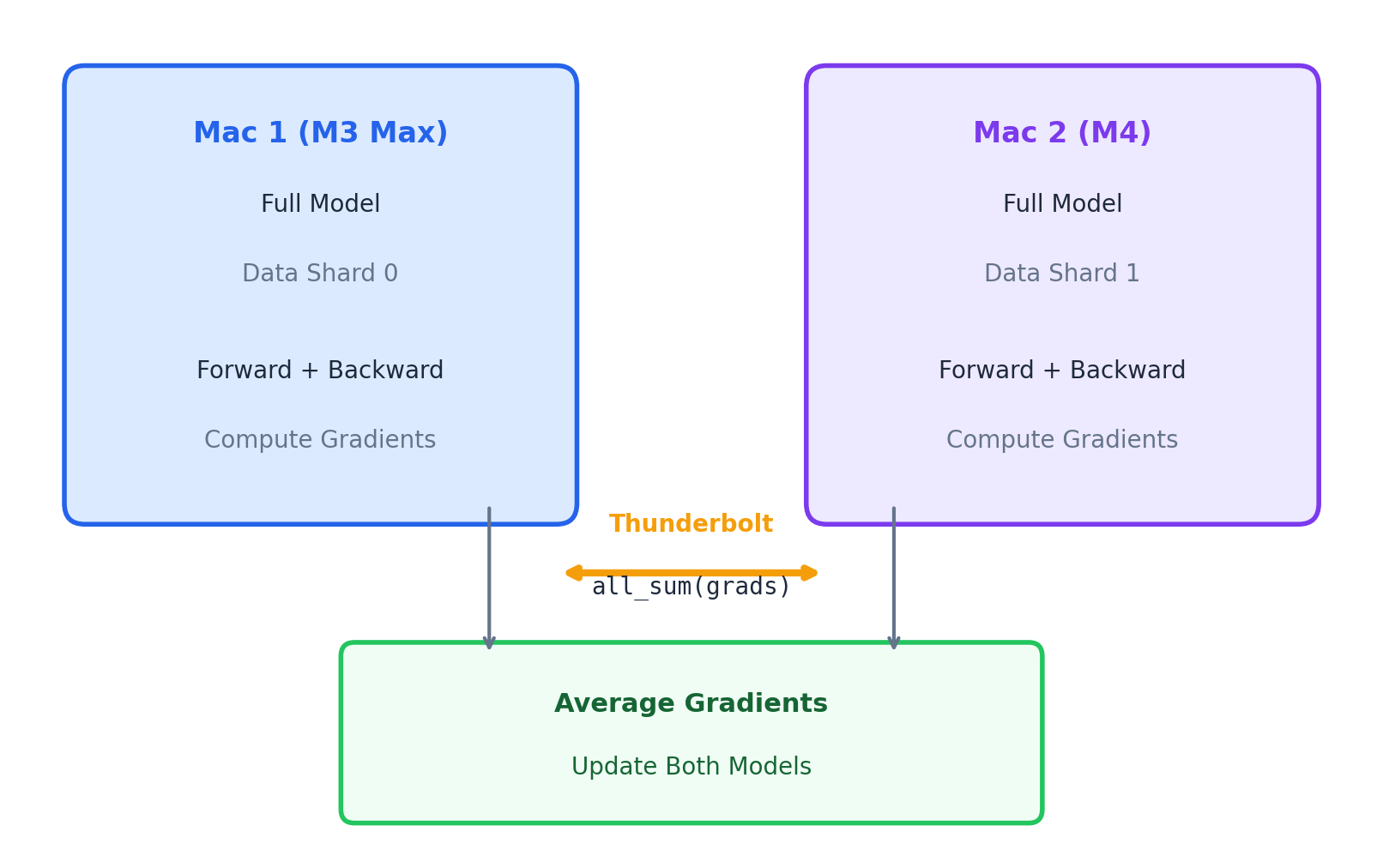
The MLX pattern for this is minimal:

import mlx.core as mx
import mlx.nn as nn

world = mx.distributed.init()
rank = world.rank()
size = world.size()

# Each rank processes different data
data_shard = full_dataset[rank::size]

# In the training loop:
loss, grads = loss_and_grad_fn(model, batch)
grads = nn.utils.tree_map(lambda g: mx.distributed.all_sum(g) / size, grads)
optimizer.update(model, grads)
mx.eval(model.parameters(), optimizer.state)

all_sum is where the Thunderbolt link earns its keep. Each gradient tensor is summed across all ranks. The result lands on every machine. At 0.4 ms round-trip, the communication overhead per step stays small for models up to tens of billions of parameters.

Data-Parallel QLoRA Fine-Tuning

We tested this with real models using mlx-lm, which has distributed support built into its LoRA training loop. The nn.average_gradients() call and rank-aware data sharding are already there. Launch with mlx.launch and the library handles the rest.

We fine-tuned two models across both Macs: Qwen3.5-0.8B (4-bit) and Liquid AI's LFM2-8B-A1B (4-bit, MoE architecture). The LFM2 has 8.3 billion parameters with 1 billion active per forward pass. It loaded on both machines at 5.35 GB per node. Val loss dropped from 7.37 to 6.94 in 10 iterations at 339 tokens/second.

Trainable parameters: 0.001% (0.053M/8339.930M)
Iter 5:  Train loss 7.649, It/sec 1.907, Tokens/sec 93.074, Peak mem 5.350 GB
Iter 10: Train loss 7.219, It/sec 7.007, Tokens/sec 339.147, Peak mem 5.350 GB

The key requirement for data-parallel QLoRA: the full model must fit on each machine individually. For 4-bit quantized models, this means models up to about 14B parameters fit on the M4 (24 GB), and up to about 20B on the M3 Max (36 GB).

Data-Parallel Inference Throughput

For inference, data parallelism means each node generates independently on different prompts. We benchmarked Qwen3.5-0.8B (4-bit, 0.65 GB per node) across both Macs:

Single node (M3 Max): 257 tok/s
Single node (M4):     142 tok/s
Cluster (1 per node): 367 tok/s
Cluster (batch=2):    964 tok/s

With batch_size=2 on each node, the cluster processes four prompts simultaneously. Total throughput: 964 tokens per second. The M3 Max is faster per-token than the M4 (different chip generations), but both contribute to aggregate throughput. For workloads like evaluating a dataset of prompts, this is a straightforward 2x speedup over a single Mac.

Memory Limits in a Heterogeneous Cluster

There's a subtlety here that's easy to miss. In a heterogeneous cluster, the node with the least memory constrains everything.

With data parallelism, each node holds the full model plus activations for its batch. The model weights are fixed, but activation memory scales with batch size and sequence length. On our cluster, the M4 (24 GB) is the bottleneck. A 17 GB model leaves roughly 7 GB for activations, optimizer states, and gradients. Push the sequence length too high and the M4 runs out of memory, even though the M3 Max has headroom to spare. You can work around this with smaller batches on the weaker node, but you can't eliminate the constraint entirely.

Tensor parallelism splits model weights across nodes. That helps with fitting larger models. But it does not split activations or the sequence dimension. Each node still holds the full activation tensor for its portion of the computation. A long sequence produces large intermediate tensors on every node. Tensor parallelism lets you run a bigger model, not a longer sequence.

Neither approach is pipeline parallelism, which splits the model by layers and passes activations between stages. MLX doesn't have a built-in pipeline parallelism API, but it can be built on top of all_sum. We cover this later in the article. For sequence-length-limited workloads within a single node, gradient checkpointing (recomputing activations during backward instead of storing them) is another lever. MLX supports this via mx.checkpoint.

Tensor-Parallel Inference

What if the model doesn't fit on a single Mac? Tensor parallelism splits weight matrices across machines. Each node holds a fraction of the parameters.

MLX provides two sharded linear layer types:

• AllToShardedLinear (column parallel): Takes full input, produces sharded output. Each rank holds output_dims/N columns of the weight matrix.
• ShardedToAllLinear (row parallel): Takes sharded input, produces full output via all_sum. Each rank holds input_dims/N rows.

In a transformer, the standard sharding pattern looks like this:

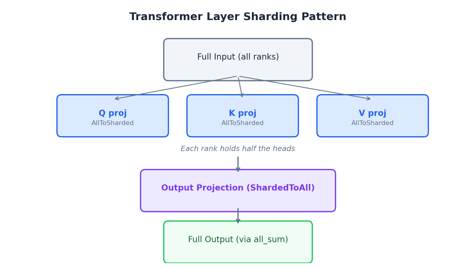
MLX's shard_inplace converts existing layers:

from mlx.nn.layers.distributed import shard_inplace

shard_inplace(attn.q_proj, "all-to-sharded")
shard_inplace(attn.k_proj, "all-to-sharded")
shard_inplace(attn.v_proj, "all-to-sharded")
shard_inplace(attn.o_proj, "sharded-to-all")

After sharding, each rank holds half the attention heads and half the FFN neurons. The combined memory of both Macs (36 + 24 = 60 GB) can support models roughly twice as large as either alone.

We verified this with a test model across both Macs:

fc1 weight shape per rank: (32, 32)
  (full would be [64, 32], each rank holds [32, 32])
Tensor parallelism PASSED!

Architecture-Specific Limitations

Not all architectures support simple tensor parallelism via shard_inplace. Liquid AI's LFM2 interleaves convolutions with projections. Shard the projections and the downstream Conv1d breaks because it expects the full dimension. Standard transformer architectures (Llama, Qwen, OLMo) work cleanly. Head splitting is orthogonal to the computation, so you're just distributing heads across ranks.

We successfully ran tensor-parallel inference on OLMoE-1B-7B (a standard transformer MoE) by sharding the attention projections and splitting the Q/K norm weights and head counts to match:

# Shard Q, K, V (column parallel)
for name in ["q_proj", "k_proj", "v_proj"]:
    shard_inplace(getattr(attn, name), "all-to-sharded")

# Split per-head norms across ranks
for norm_name in ["q_norm", "k_norm"]:
    norm = getattr(attn, norm_name)
    chunk_size = norm.weight.shape[0] // size
    norm.weight = norm.weight[rank * chunk_size:(rank + 1) * chunk_size]

# Shard output (row parallel)
shard_inplace(attn.o_proj, "sharded-to-all")

# Update head counts
attn.n_heads = attn.n_heads // size
attn.n_kv_heads = attn.n_kv_heads // size

Sharded LoRA: Tensor-Parallel Fine-Tuning

This is where we went beyond what MLX currently offers.

Standard LoRA adds low-rank adapters to frozen base model layers:

# Standard LoRA forward pass
y = self.linear(x)                      # frozen base
z = (self.dropout(x) @ lora_a) @ lora_b # trainable adapter
return y + scale * z

mlx-lm's LoRA checks isinstance(layer, nn.Linear). Sharded layers aren't nn.Linear subclasses, so LoRA refuses to wrap them. Even if it could, the shapes wouldn't match. If the base linear produces sharded output, the LoRA path needs to produce matching sharded output.

We implemented two new classes to solve this. The column-parallel case is shown below:

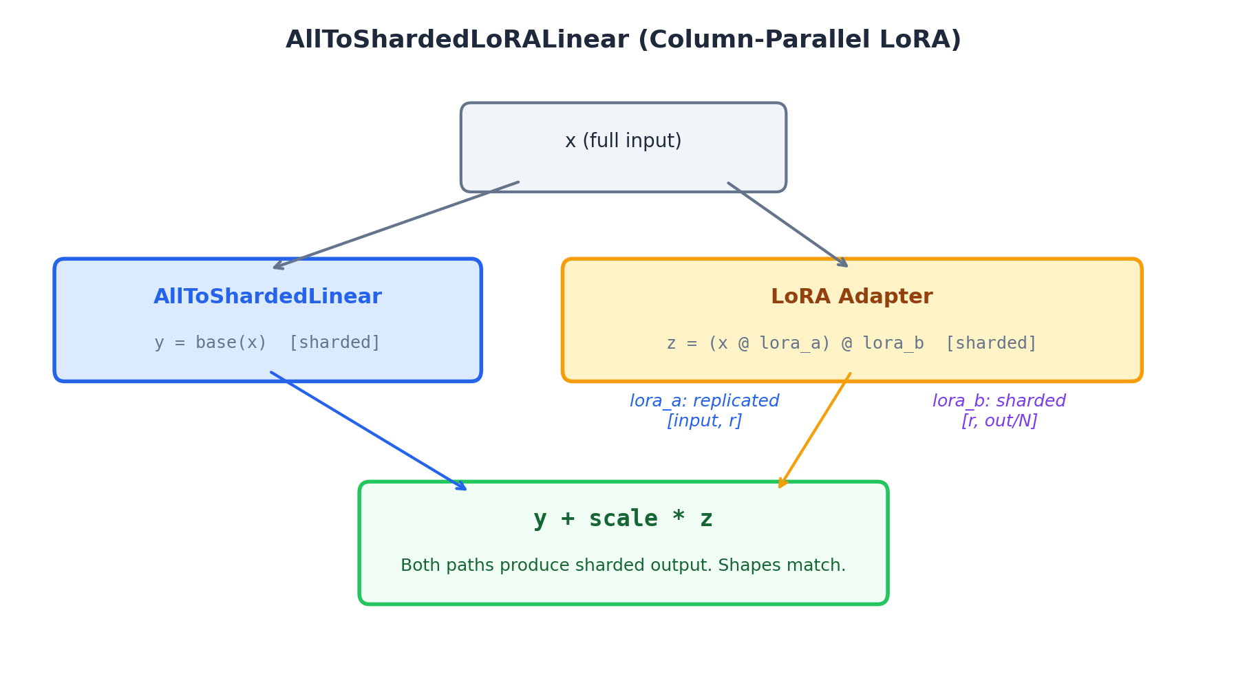
AllToShardedLoRALinear (Column-Parallel LoRA)

For layers where the base linear splits output across ranks:

Input: full (same on all ranks)
Base output: sharded (each rank gets output_dims/N)
LoRA must also produce: sharded output

• lora_a is replicated: shape [input_dims, r], same on all ranks
• lora_b is sharded: shape [r, output_dims/N], each rank holds its slice

def __call__(self, x):
    y = self.linear(x)  # AllToShardedLinear
    # sum_gradients: identity forward, all_sum backward
    # ensures replicated lora_a gets aggregated gradients
    lora_a = sum_gradients(self.group)(self.lora_a)
    z = (self.dropout(x) @ lora_a) @ self.lora_b
    return y + (self.scale * z).astype(x.dtype)

ShardedToAllLoRALinear (Row-Parallel LoRA)

For layers where the base linear gathers sharded input into full output:

Input: sharded (each rank gets input_dims/N)
Base output: full (after all_sum internally)
LoRA must also produce: full output

• lora_a is sharded: shape [input_dims/N, r], each rank's input slice
• lora_b is replicated: shape [r, output_dims], same on all ranks

def __call__(self, x):
    y = self.linear(x)  # ShardedToAllLinear (has internal all_sum)
    # sum_gradients ensures replicated lora_b gets aggregated gradients
    lora_b = sum_gradients(self.group)(self.lora_b)
    h = self.dropout(x) @ self.lora_a  # partial
    z = h @ lora_b                      # partial
    z = mx.distributed.all_sum(z, group=self.group)  # aggregate
    return y + (self.scale * z).astype(x.dtype)

The Gradient Synchronization Problem

The core challenge: gradient correctness. In each class, one LoRA matrix is replicated (same on all ranks) and one is sharded (different per rank). The replicated matrix must receive identical gradient updates on all ranks to stay synchronized.

MLX's sum_gradients() solves this. It's identity in the forward pass. It performs all_sum in the backward pass. Wrap the replicated parameter through sum_gradients before use, and its gradient is automatically aggregated across ranks during backpropagation. No manual gradient synchronization in the training loop.

For AllToShardedLoRALinear: lora_a (replicated) goes through sum_gradients. lora_b (sharded) doesn't need it. Each rank's gradient is already correct for its shard.

For ShardedToAllLoRALinear: lora_b (replicated) goes through sum_gradients. lora_a (sharded) doesn't need it.

End-to-End Verification

We verified sharded LoRA training across both Macs with a transformer block where attention projections are sharded and LoRA adapters are applied to Q and V:

=== Sharded LoRA Test (2 nodes) ===
AllToShardedLoRALinear: PASSED
ShardedToAllLoRALinear: PASSED
End-to-end training losses: ['2.0248', '2.0236', '2.0216', '2.0190', '2.0157']
Loss decreasing: True
End-to-end sharded LoRA training: PASSED!

We then tested on real models. OLMoE-1B-7B (6.9B parameter MoE) with tensor-parallel sharded LoRA across both Macs:

============================================================
Tensor-Parallel QLoRA - OLMoE-1B-7B (2 nodes)
============================================================
Model loaded: 1,081,231,360 params
Sharded 16 projections, 8 LoRA adapters
Trainable: 196,608 / 1,076,176,896 (0.0183%)

Training for 10 steps...
  Step 5/10 | loss: 2.4513 | time: 1.16s
  Step 10/10 | loss: 1.7190 | time: 1.72s

Tensor-parallel QLoRA complete! (1.7s)
Peak memory per node: ~4.11 GB

Handling Quantized Models

One thing that tripped us up: when QuantizedLinear is sharded via shard_inplace, the weight shape reflects quantized dimensions, not logical ones. A 4-bit layer with logical shape [6144, 2048] has actual weight shape [6144, 256] (because 2048 * 4 / 32 = 256 packed int32 elements). The from_base method needs to correct for this:

output_dims_per_rank, input_dims = linear.weight.shape
if hasattr(linear, "bits"):
    input_dims = input_dims * 32 // linear.bits

Without this correction, the LoRA matrices are created with the wrong dimensions and the first forward pass crashes with a shape mismatch.

Distributed Batch Inference

For evaluating models across both Macs, we split problems across ranks and use batch_generate for additional throughput within each node.

The optimal configuration for our heterogeneous cluster:

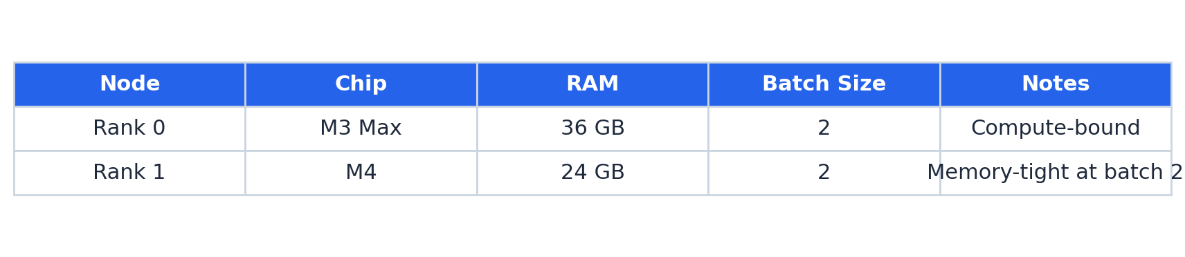
We tested batch size 3 on the M3 Max (it has the headroom). Generation is compute-bound, not memory-bound. Time per problem actually increased because the model generates 3x the tokens per batch with no parallelism in autoregressive decoding.

With batch_size=2 on both nodes processing different problems:

RESULTS: 5/12 (41.7%)
Time: 599s (49.9s/problem)
Effective throughput: 1.2 problems/min

This gave us ~72 problems per hour, enough to evaluate large validation sets overnight while iterating on training strategies.

Practical Tips

After every reboot:

1. Run ssh-add --apple-use-keychain ~/.ssh/id_rsa (or configure ~/.ssh/config with UseKeychain yes)
2. Log in to the other Mac physically (FileVault blocks SSH before login)
3. Check bridge0 IPs (they change every time)
4. Update hosts_tb.json with the new IPs
5. If mlx.launch gives "bind error 49", use -p 3700 or another port

Installing packages on both Macs:

.venv/bin/pip install <package>
ssh bob@mac2.local \
  "cd projects/dist-mlx && .venv/bin/pip install <package>"

Debugging distributed runs: Add --verbose to mlx.launch to see ring connection logs. If rank 1 shows "error: 65" (EHOSTUNREACH), your bridge0 networking is broken. Probably from a previous ifconfig bridge0 deletem or a cable disconnection. Reboot both Macs.

Memory planning for 4-bit models:

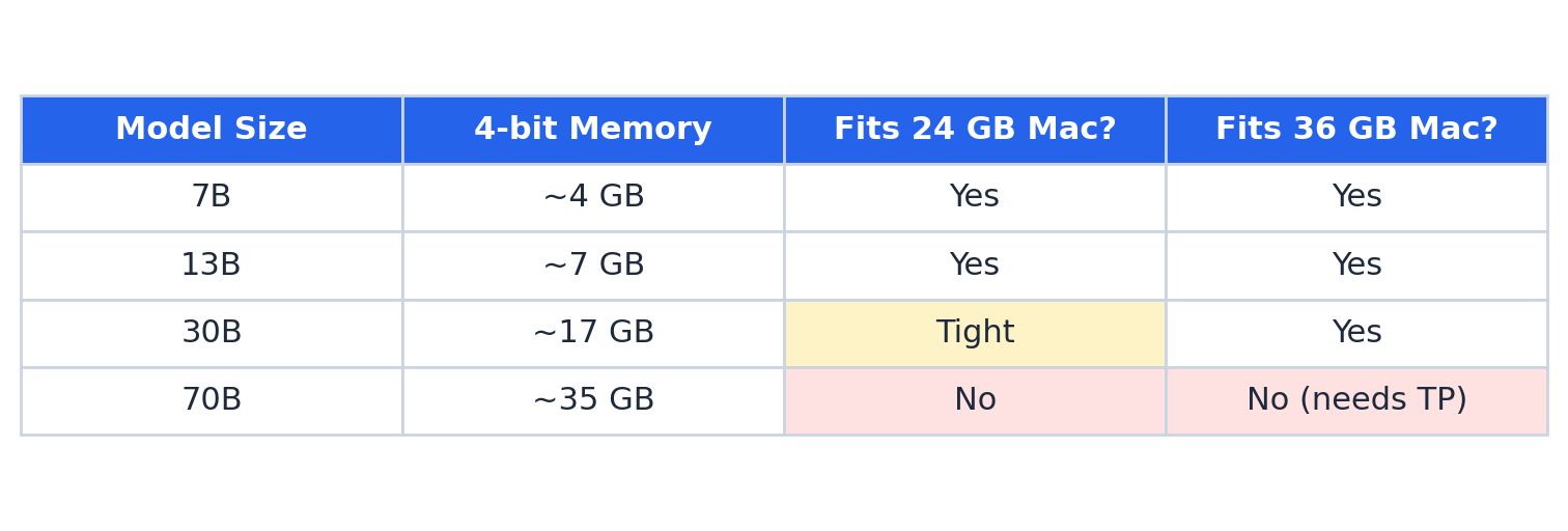
With tensor parallelism across both Macs, you effectively double the memory available for model weights. A 70B model at 4-bit (~35 GB) could be split ~18 GB per node, fitting on both machines. Keep in mind: this doubles weight capacity, not activation capacity. Each node still needs memory for the full activation tensors at its layer boundaries.

Pipeline-Parallel Inference

Data parallelism replicates the full model on every node. Tensor parallelism splits weight matrices but keeps full activations on every node. Pipeline parallelism does something different: it splits the model by layers. Rank 0 runs the first half of the transformer stack. Rank 1 runs the second half. Activations flow from one to the other.

This matters because both weights and activations are split across nodes. Each node only stores the KV cache for its layers. For long-context inference, where the KV cache dominates memory, this is the difference between fitting and not fitting.

MLX has no built-in pipeline parallelism API. But it has all_sum, and that's enough. The trick: rank 0 computes its layers and produces real activations. Rank 1 creates a zero tensor of the same shape. Both call all_sum. The result is rank 0's activations on both nodes (zeros + values = values). Rank 1 then feeds those into its layers.

# Rank 0: compute first half
if rank == 0:
    h = embed(tokens)
    for layer in layers[:mid]:
        h = layer(h, mask=None)
    mx.eval(h)
else:
    h = mx.zeros((B, L, d_model), dtype=mx.bfloat16)
    mx.eval(h)

# Sync barrier (ensures both ranks are ready)
mx.eval(mx.distributed.all_sum(mx.array([1.0])))

# Transfer activations: zeros + real values = real values
h = mx.distributed.all_sum(h)
mx.eval(h)

# Rank 1: compute second half
if rank == 1:
    for layer in layers[mid:]:
        h = layer(h, mask=None)
    h = norm(h)
    logits = lm_head(h)

One critical detail: the placeholder zeros must match the activation dtype exactly. The model outputs bfloat16. If you create float32 zeros, all_sum silently hangs. No error, no timeout, just a deadlock. We lost time on this.

We tested pipeline parallelism with two models. First, Qwen3.5-0.8B to verify correctness:

Pipeline Parallel LLM Inference (2 nodes)
Model: 24 layers, d=1024
  Rank 0: embed + layers 0-11
  Rank 1: layers 12-23 + norm + head

Prompt: 'The capital of France is' (5 tokens)
Pipeline next token: ' Paris' (id=11751)
Pipeline parallel inference PASSED!

The output matches what the full model produces on a single node. Then we ran Nemotron-3-Nano-30B (31.6B parameters, 17.8 GB at 4-bit) in pipeline mode. This is the kind of model where pipeline parallelism earns its keep. At 17.8 GB, it fits on the M3 Max (36 GB) alone but leaves the M4 (24 GB) with only 6 GB headroom for activations. Split across both nodes, each holds 26 layers and 17.9 GB peak, leaving comfortable room on both machines.

Loaded. 52 layers, d=2688
Memory: 17.78 GB
Rank 0: embed + layers 0-25
Rank 1: layers 26-51 + norm + head
  ctx=98: 0.42s
Peak memory: 17.92 GB per node

Comparing All Three Parallelism Modes

Each mode splits the workload differently, with different tradeoffs for your heterogeneous cluster:

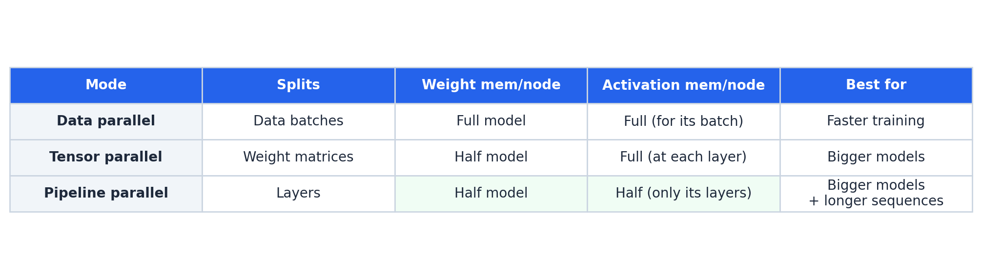
Pipeline parallelism has higher per-token latency (sequential through the pipeline), but it's the only mode that reduces both weight and activation memory per node. For a 70B model at 4-bit with 32K context, where neither weights (~35 GB) nor KV cache (~8 GB) fit on the M4 alone, pipeline parallelism puts ~17.5 GB weights + ~4 GB KV cache on each node. That fits.

What's Next

The sharded LoRA implementation described here is, to our knowledge, the first working tensor-parallel LoRA for MLX. The changes needed in mlx-lm are small: a new to_lora case in linear_to_lora_layers for sharded linear types, plus the two wrapper classes. Models that already support MLX's shard() method (Llama, Qwen, Mistral) would get tensor-parallel LoRA for free.

Apple Silicon Macs, even consumer-grade ones, can form useful training clusters over Thunderbolt. The 0.4 ms latency is low enough that gradient sync doesn't bottleneck training for most model sizes. With macOS 26.2's RDMA support over Thunderbolt 5, the next generation of this setup could see communication latency drop to 50 microseconds. That starts closing the gap with datacenter interconnects.

Two MacBooks and a cable is enough to get started.

All code shown in this article is self-contained. The sharded LoRA classes (AllToShardedLoRALinear and ShardedToAllLoRALinear) can be dropped into any MLX project as a single file. The hostfile, launch commands, and training patterns work with MLX 0.31.1 and mlx-lm 0.31.1 on macOS 26.x.