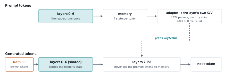
Cut a trained model at a chosen depth. The lower layers will read the prompt and pass on a projected memory to the higher layers. This cuts down the cost of processing the prompt by 4x. But they also failed to catch any of their metrics!
A 24-layer language model will read your 16,000-token document 24 times before it even starts talking. Send a long prompt to it, and watch how quickly it gets its first word – on long prompts, time-to-first-token can be very slow.
A strange way to use compute in transformers is that the upper layers mostly decide what to say next, while the lower layers are responsible for reading the input. So they asked themselves: what if only the lower layers saw the prompt, but the upper layers got a summary instead?
The cut
Take a pretrained model and choose a depth, say layer 7 of 24. Everything below that is the reader; it processes the prompt once and outputs a residual stream which is the memory for each prompt token. Everything above never sees the prompt.
At each of its attention layers, a small adapter maps the memory into the keys and values the layer would compute for itself, and those are prepended to the cache. The model is then healed by continuing pretraining, since it has been changed in terms of how information flows through it.
We call this model grafting. The name can change depending on what you’re trying to graft: swapping softmax attention for a linear variant and retraining is a graft; splitting a feedforward layer into experts and adding a router is a graft; turning an autoregressive model into a diffusion one by annealing its attention mask is a graft. No two grafts are exactly the same.
Diffusion conversion (DC) is a technique that converts diffusion models into transformers by changing their causal mask. DC can be used to upconvert a model from a pure diffusion model to a transformer model, or vice versa. This process costs 200-580 billion tokens.
Upcycling to a mixture of experts (MoE) replaces each token with a different router, costing about half the cost of pretraining a diffusion model. Our graft leaves generate tokens on the path they’re trained for and divert only prompt tokens – costing half a billion. Three orders of magnitude, one quantity.
One detail of our graft we have not seen elsewhere: the adapter does not predict keys and values. Instead, it maps memory into the input space of the host layer, which then performs its own projections. Initialise the adapter to the identity and the first graft site is bit-exact with the original model at step zero. This works for a 0.8B model with 5.2M parameters.
What the benchmarks said
We grafted Qwen3.5-0.8B-Base and healed it on 500M tokens of FineWeb-Edu.
Validation loss came out at 2.613 vs. 2.645 for the original 500M tokens of pretraining. Passkey retrieval from a 32K prompt held at 99% (control: 99%). HellaSwag through MMLU scored 0.580 (vs. 0.581 for the control). Decode throughput remained unchanged - generated tokens still cross the full stack.
And the prompt got cheap. Time-to-first-token improved 2.1x (at 16K tokens) and 4.0x (at 128K) on an A40, measured end to end, compared to estimates based on parameter count alone. Forward hooks also show that layers 7-23 only get one token at a time during generation - no prompt ever! 153M parameters run per prompt token vs 498M for the baseline.
At that point we had a model that looked finished.
The tool test
Long-context evaluation has a bad habit: our retrieval test hid a nine-character key like 1234-5678 in a long document and asked for its value; the grafted model got 0.90.
Then build a test shaped like the thing you care about: put eight tool schemas in a long prompt labeled [t0] through [t7], ask for a call to t5, and make sure the model finds one of those lines and reproduces the correct multi-token function name and arguments.
The original model gets 0.97. The grafted one got 0.27.
Every other number was fine. Validation loss beat the baseline. Capability average was at parity. Passkey retrieval was 99%. It would have been shipped.
Two things about the diagnosis are unexpected: it’s not a copying failure; the model emits well-formed real function names with valid argument keys, but only eight tool names are wrong (one is a mis-copy). It’s also an indexing failure – our old test passes because 1234-5678 is distinctive enough to tell t5 from t4.
Feed the upper layers mathematically perfect memory, lift the true hidden states out of the frozen original, and the graft starves for nothing. The query is what’s starving, not the keys. It requires several rounds of prompt-conditioned computation to form a sharp enough question, but there are no graft sites in between.
Getting it back
Two fixes work. The first is data, and we nearly missed it.
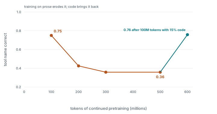
Indexing does not break when you graft so much as bleed away while you heal. At 100M tokens of FineWeb-Edu, the model scores 0.75. At 200M, 0.43. At 500M, 0.36. Validation loss improves the whole way down. Prose has almost no “find the item labelled X and reproduce it exactly” structure in it – half a billion tokens of it makes the model stop using circuits at all.
Resume that degraded checkpoint for 100M tokens with 15% code mixed in and it returns to 0.76. Thirty percent gets 0.79, inside the noise, so the curve is steep to fifteen and flat after; the whole repair costs four thousandths of a nat on prose validation loss.
HumanEval goes from 0.183 to 0.189 during this whole repair. It's because HumanEval doesn't really care about what the code data was fixing - it just looks at how much better the code runs compared to random code.
The second fix is to freeze. Resume the same checkpoint for 100M tokens of deliberately pure prose. It goes from 0.75 to 0.43 when all layers are trained; with the upper seventeen layers frozen, it’s 0.69. Validation loss improves slightly, but peak memory drops from 23.5 GB to 16 GB.
One caveat with the term “freezing” is that it does two things in this literature: the encoder must continue training (it’s the part that writes the memory), and the layers above the graft should stay frozen.
Where to cut
This is the real design decision and it is a frontier, not a value.
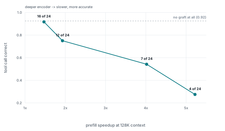
Four fresh grafts, each 100M tokens on the corrected recipe, differing only in where the model was cut:
| encoder | params per prompt token | tool call correct | prefill at 16K | at 128K |
|---|---|---|---|---|
| 4 of 24 | 88M | 0.28 | 2.94x | 5.22x |
| 7 of 24 | 153M | 0.54 | 2.11x | 4.02x |
| 12 of 24 | 252M | 0.75 | 1.56x | 1.93x |
| 16 of 24 | 334M | 0.92 | 1.27x | 1.47x |
| no graft | 498M | 0.92 | 1.00x | 1.00x |
At 16 out of 24 the graft matches the control exactly and gives 1.5x on a 128K prompt. At 7 out of 24 you get 4x, but the model can't reliably call tools. This is a good product, but it's not the same as the other one. If you're using a summariser or a long-document reader, go with the 4x. Anything that does tool calls should be deeper than this.
Three things that did not help
The null results taught us more than the wins.
Alignment losses. Regressing adapter output onto the original model's true hidden states, as an auxiliary term, slightly hurt: 0.71 against 0.75 at matched tokens.
Projector capacity. We tested this one hard, because the obvious objection to a 5.2M adapter is that it is too small.
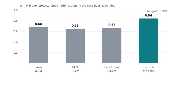
Freezing the base model and training only a projector for dense key-value regression, they achieved an eleven-fold capacity range of 3.2M linear maps, 12.6M per-token MLPs, and 34.6M causal transformers with their own sequence mixing, all running at two different learning rates. Their results were 0.59 - 0.68 across all three models; the MLP had the best regression performance but the worst downstream accuracy. You can drive approximation error down without buying the capability: fidelity of the keys wasn't the bottleneck.
Code data as a HumanEval fix. Fifteen million code tokens moved HumanEval by 0.006 and full tool calls by 0.37. It turned out that the code slice was too small to be worth measuring.
Limits
One model at one scale: everything here is Qwen3.5-0.8B. No matter how big or small your GPU is, nothing in this codebase cares about scale. A 9B graft will fit on a single 48 GB card.
The tool probe is synthetic (it's not BFCL). The base model is not instruction-tuned, so it will score near the floor on any task that doesn't involve grafting.
Qwen3.5 uses six full-attention layers, so cutting at 16 leaves only two layers above the cut (and thus little quadratic work skipped). The layer layout of Qwen3.5 is such that models with an attention-to-recurrent ratio other than 16 sit somewhere along this curve.
Twenty trials per cell puts roughly ±0.1 of noise on the copy numbers. Trust the monotonic ordering across four depths, not any single gap.
Prior work
The design is not ours: DeepSeek-V4.1-Flash is a causal encoder-decoder that projects the decoder's key-value cache from the encoder's final hidden state, trained from scratch on 45T tokens. YOCO published the early-exit-during-prefill structure before that. The conversion is not ours either. LLKVApprox retrofits this onto frozen checkpoints with a projector and a 256-token exact suffix. We arrived at a 256-token tail separately, which says the number is probably right. It does not make it ours.
Grafting - one operation with a cost law predicting its price; a swept speed-versus-capability frontier (instead of a single chosen depth); the forgetting effect and its repair; a projector 180 times smaller than the other, because it reuses the host layer's own projections.
And the evaluation result – the most portable of all metrics. It’s possible for a model to improve on validation loss, keep its benchmark average, retrieve from 32K, but lose the ability to distinguish between two similar labels. If you’re grafting something, measure it first!
Next
A final run on the recipe this study found: freeze the upper layers, train the encoder, add 15% code to the mix, use a 256-token tail, and choose the split based on workload (not default). The resulting 9B graft is now affordable, and they’ve also trained an instruction-tuned model for a real tool-calling benchmark.