They built a public benchmark for typed model decisions, tested a frozen 149M encoder with twenty small classifier heads on it, compared the result to TypeSafe’s Jev, and fixed two bugs in their classifier library.
Much of what software asks a language model for is a yes/no question (e.g., “Is this ticket about billing?”). It’s also common for models to be asked to write paragraphs that are then parsed into answers, such as when a user wants to know whether a security alert needs a human to review.
TypeSafe ships a model, Jev, built for that job. It takes unstructured state and returns typed decisions with probabilities attached. There are three kinds: a yes/no question returns a probability, a choice returns a distribution over labels, and a score returns a distribution over the levels of a rubric. A single call answers all the questions asked about one piece of state.
We couldn't find a public benchmark for this kind of output, so we created one ourselves and tested the smallest model we could think of on it.
What one case looks like
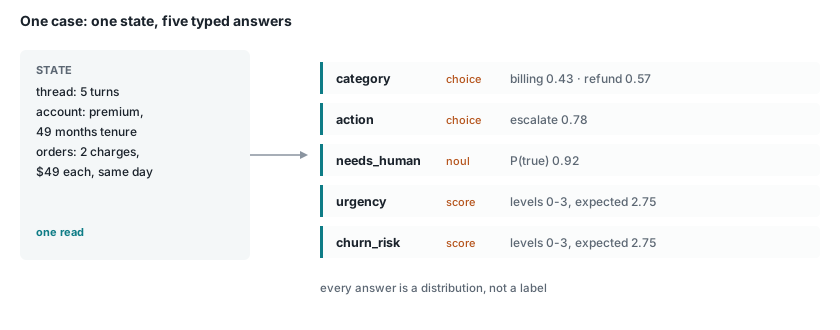
Each case is a piece of state – a customer thread for an account, a security alert for a machine’s history, or a vendor invoice for a purchase order and delivery note.
Each case contains five questions that mix up the three types of labels. Each option is accompanied by a written description (which is part of the input).
The gold answers are probability distributions. For each case, you sample a teacher model three times and average those three distributions (instead of voting on them). The gold is sharp where the teacher is consistent and soft where it disagrees with itself. You also score the label and the distribution together – the probability that the teacher assigns to a given typed decision is part of the answer.
The test set contains 400 cases and 2,000 decisions for each of four workflows, all held out. The training data is generated in a separate run with a different seed.
The benchmark we had to throw away first
Our first version of the benchmark was broken, and it took us a while to see it.
It had 5,000 cases with only 105 distinct input strings (each appearing in all three splits). Four of its five decisions had been sampled independently of the input; therefore, none could beat the base rate. It was still tied for first place until now.
The replacement checks for that failure: each case is built from sampled latent factors, and an audit measures the mutual information between those factors and the gold labels (as a fraction of label entropy). The broken version scored near zero on this measure; the published set has values ranging from 0.119 to 0.850 across its twenty questions, with no question collapsing onto a single answer and every state being distinct.
The audit is cheap to run, and we would recommend it to anyone building a synthetic benchmark.
The encoder baseline
The baseline uses Adaptive Classifier, a library that combines a prototype memory of examples with a small neural head, both on top of a frozen sentence encoder. Nothing in it is generative. We trained one classifier per question, twenty in all, on 300 cases each.
Two reference points help in reading the results.
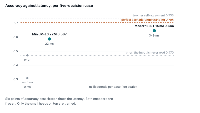
A model that ignores the input and just answers with each question’s training frequencies scores 0.470 (the floor). A model that recovers every case’s latent factors perfectly would score 0.704, but this is an optimistic upper bound because the factors contain information the text doesn’t.
A 22M encoder at 22 ms/case gives 0.587 (half way up), and a 149M encoder at 349 ms/case gives 0.646 (three quarters up).
On the ordinal questions the bigger encoder lands within one rubric level of the teacher 93% of the time.
The larger encoder buys six points of accuracy for sixteen times the latency: both run on a laptop.
We also wanted to know how a model built for this task would do. Once we had API access, on 18 September, we ran Jev on all 400 cases: 2,000 decisions with no errors, at 710 milliseconds per case and 16 cents in total.
Jev scores 0.727, which is eight points above the larger encoder (factor ceiling = 0.735) and only 0.008 below the teacher's self-agreement ceiling (0.735). Jev therefore has very little room to improve on accuracy at this benchmark.
Jev has never seen the twenty question schemas used to train the encoders. Jev’s encoders are trained on the same four workflows that they’re tested on, but can’t answer questions outside those workflows.
The distributional comparison came out differently.
| accuracy | KL from gold | |
|---|---|---|
| ModernBERT-base, 149M frozen | 0.646 | 0.223 |
| Jev 1.13.0 | 0.727 | 1.442 |
Jev picks the right label more often, but its KL divergence from the gold distribution is about six times the encoder's. It tends to put nearly all of its probability on one answer. The encoder is right less often, but when the three teacher samples split two to one, its probabilities split in a similar way.
Jev’s expected calibration error is 0.144 (with an overconfidence component of just 0.023), meaning its confidence in its predictions largely comes from how often it’s right. This is because Jev uses three teacher samples to encode the spread of gold, but you can’t know about this spread unless you have access to all three teachers.
Jev is eight points better when routing on the top label. Rank by the probability of being above the threshold, or pass it to a downstream step that multiplies it. The 149M encoder (a 2024 model) tracks the teacher’s uncertainty much better than KL=0.223 vs 1.442.
One caveat to this score is that it measures agreement with your teacher (not correctness). If Jev is right but your 4B-class teacher is wrong, Jev gets penalised for it, so the true accuracy advantage of 0.727 may be overstated.
Two bugs in the classifier library
The first run of the larger encoder scored 0.477 (just over the input-blind floor of 0.470) and on one five-option question scored 0.180 (below the 0.200 expected by chance).
The library reduces every model’s token embeddings to a single vector by taking the CLS token (for example, for most encoders this is the wrong choice). The library is most often used with all-MiniLM-L6-v2, which has a config setting “mean pooling” – meaning it trains the model on mean pooling rather than training CLS as a sentence representation.
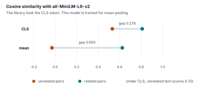
On ordinary sentence pairs, CLS pooling gives unrelated texts, such as a sentence about a man playing guitar and one about an invoice paid late, a cosine similarity of 0.53. Mean pooling puts the same pair near zero and makes the gap between related and unrelated pairs 2.4 times wider.
The prototype memory uses nearest-neighbour search to find the most similar vector for each class. As all the vectors are packed into a narrow band of high similarity, the prototypes can no longer distinguish between classes and they were pushed down towards zero by the tuning.
We found the second bug while tuning around the first: the library exposes prototype_weight and neural_weight to control how much each signal counts. They are both read from the config and stored on the object, but not used. Two prediction paths each hardcoded their own 0.7 and 0.3, so they could disagree with each other when the config was changed. Other keys like epochs and batch_size had the same issue.
Both bugs are fixed in release 0.2.0. Pooling now defaults to whatever the model's config says it was trained with, and classifiers saved before the change keep their old pooling when loaded, so upgrading does not silently change anyone's predictions.
The pooling fix alone took the larger encoder from 0.477 to 0.565.
Training on the distribution
The gold is a distribution, but the library trains on hard labels, so the soft target was being discarded during training.
A classifier that only accepts labels can still learn a distribution from replicated examples. We entered each case several times and split the copies across labels in proportion to its gold distribution, so a case the teacher called 70/30 became three examples of one label and one of the other. We used largest-remainder apportionment so that rounding does not lose any copies.
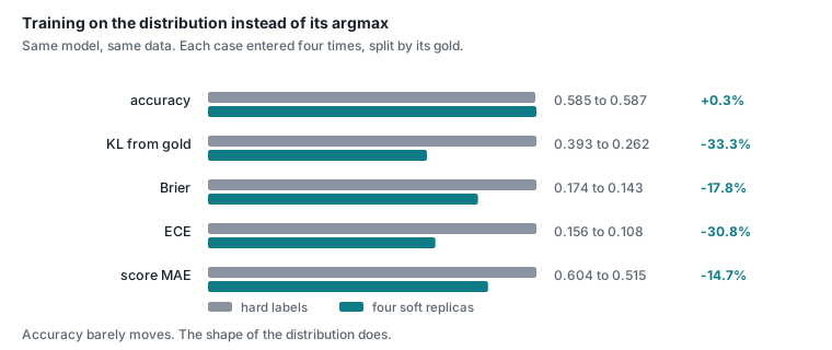
Accuracy barely moved, from 0.585 to 0.587. KL divergence from the gold fell by a third, the Brier score by 18%, calibration error by 31%, and error on the ordinal questions by 15%.
The top labels were already mostly right; what improved was the probability attached to them.
The cost is roughly seven times the training time, because the encoder embeds four identical copies of every text and the library does not cache embeddings. Training happens offline, so we accepted that.
What this does not show
Gold (a score measuring agreement with a teacher) was calculated for a model of roughly 4B capacity, trained three times. Gold doesn't measure correctness; the teacher may be wrong in some cases – e.g. missing a duplicate invoice whose number exactly matches an earlier one.
A fresh teacher sample is 73.5% correct when compared to gold (the other samples), meaning a score higher than this means you’re predicting the teacher’s habits instead of answering the question correctly. If your model scores lower than the teacher, then every time it answers correctly where the teacher answered incorrectly, it earns points against its total score.
States are generated rather than drawn from real support queues or SIEM logs. The encoder that generates states is trained on the workflow of the system it’s scoring, and therefore cannot answer questions about other systems. The other encoder (Jev) can accept any schema for state data at runtime, but the specialist encoder is better suited to answering questions about its own workflow.
Conclusion
A frozen 149M encoder with twenty small heads recovers three quarters of the learnable signal in a larger model’s typed decisions in about a third of a second on a laptop. A 22M version recovers half of it in just 22 ms. Jev is more accurate than both, and its probabilities track the gold distribution much better.
For decisions that software makes constantly, often by calling a frontier model, that is a better trade-off than we expected.
The benchmark is public, and so are the library fixes and the reference scores, so new results can be compared against the floor, the ceiling, and the models reported here.